
How We Decode the Math Behind the Market
The Cycle Map

How We Decode the Math Behind the Market
The Cycle Map
Every asset in the covered universe is classified by a machine-learning model into one of six cycle phases, refreshed on the monthly close.
The model does not predict price. It reads structure, volatility regime, momentum persistence, participation, trend integrity, and answers a different question: where in the cycle is this asset standing right now, and what does that phase historically do to the payoff distribution?
Capital enters at the open of Phase 2 and leaves at the open of Phase 6. Everything between is governance, not opinion.
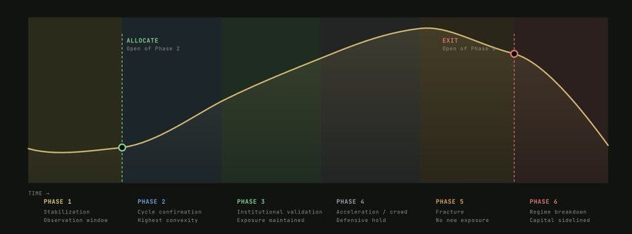
Phase 1/6: Stabilization
Prices stabilize after a prolonged decline. Volatility compresses and downside momentum weakens, suggesting early balance between buyers and sellers. Informed capital begins to re-enter, typically before broad confirmation.
This is a pre-allocation observation window. Risk remains elevated, but marginal downside is declining and early structural repair becomes visible.
→ No allocation. A monthly close in Phase 1 prepares entry in the next phase.
Phase 2/6: Positive Cycle Confirmation
The beginning of the positive cycle: the confirmed positive-cycle candle appears. Trend structure shifts decisively upward, offering the most favorable asymmetry between expected return and downside risk across the whole cycle.
The highest convexity point, risk-adjusted returns are maximized and the probability of large drawdowns is lowest relative to future upside.
→ Capital is allocated at the open of this phase and maintained through it.
Phase 3/6: Institutional Validation
Institutional participation confirms the uptrend. Liquidity improves, breadth expands, and trend persistence becomes statistically robust.
The cycle moves from probabilistic to structurally validated. Expected returns remain positive, but governance shifts from entry optimization to risk management.
→ Exposure maintained, capped by the Exposure Ceiling as the phase and the edge are re-read each month.
Phase 4/6: Acceleration
Momentum accelerates as media exposure increases and retail participation expands. Price extensions become more aggressive and increasingly detached from fundamental repricing.
Return potential may persist, but risk asymmetry deteriorates: price behavior becomes sentiment-driven rather than structurally supported.
→ Positions held defensively. No capital added. The ceiling contracts as asymmetry deteriorates.
Phase 5/6: Fracture
The uptrend begins to fracture. Volatility expands, price behavior becomes erratic, and downside risk accelerates.
Trend integrity deteriorates and the return distribution shifts unfavorably, with drawdown risk dominating expected return.
→ Minimal exposure. A monthly close here prepares the exit at the next open.
Phase 6/6: Regime Breakdown
Structural weakness confirms the end of the positive cycle. Participants remain invested despite clear regime deterioration.
A capital-at-risk environment where recovery expectations are no longer supported by probability or structure.
→ Positions exited at the open. Capital stays sidelined until a new Phase 1 emerges.
The Two Numbers on the Sheet
The phase tells you where an asset is. It does not tell you whether being there pays, or how much capital the position deserves. Those are two separate questions, and each has its own equation.
ζ‑X — Mathematical Expectancy
Zeta‑X is the expectancy of the asset in its current phase: how much you can expect to make, on average, per dollar risked. It is probability multiplied by payoff, not probability alone.

The counterintuitive part, and the reason expectancy is the number that matters: how often you win is not the most important factor. A strategy that wins most of the time can still be a losing strategy if the average loss is larger than the average win. And a strategy that loses more often than it wins can still compound wealth if the payoff is tilted far enough in your favor.
Probability is the part of the equation you cannot control, the future is unknowable. Payoff is the part you can: risk management cuts the size of the losses, position sizing scales the size of the wins. That is where the edge lives.
HOW TO READ IT:
Positive ζ‑X — the asset, in this phase, carries a positive expected payoff per dollar risked.
Negative ζ‑X — the payoff distribution is tilted against the holder. No capital is committed.
0.00 / n/d — no allocable expectancy, or insufficient data for the engine to read.
Exposure Ceiling: Kelly Criterion
Expectancy answers is this worth risking capital on. It says nothing about how much. That second question is a sizing problem, and sizing has a mathematically optimal answer: the Kelly criterion (J. L. Kelly Jr., Bell System Technical Journal, 1956), the fraction of capital that maximizes the long-run compound growth rate of the portfolio.

The Exposure Ceiling is that fraction, computed from the asset’s ζ‑X (the edge) and then conditioned on the cycle phase, because the same edge does not deserve the same capital in Phase 2 as it does in Phase 5. Bet the full Kelly fraction and volatility drag will eventually punish the estimation error in p and b; Zurique runs a fractional Kelly and treats the output as a ceiling, not a target. It is the maximum weight the math permits, never a minimum, never an instruction to fill it.
Risk is controlled here. Not at the exit, not at a trigger price, at the size of the position itself. The ceiling is re-read every monthly close: as the phase advances and the payoff asymmetry deteriorates, the permitted weight contracts, and at the end of the cycle it goes to zero.
HOW TO READ IT:
Negative or absent expectancy → Kelly returns zero or negative → the ceiling is 0%. The math refuses the position.
Phase 1 or 6 → no new exposure is permitted regardless of the edge.
A high ζ‑X in a late phase does not buy a high ceiling. Phase governs.
Kelly fraction and phase conditioning are proprietary to the Zeta engine.